
The honest answer is between 3 months and 5 years, which is useless on its own.
So let’s make it useful. This piece breaks down where the time actually goes, which factors stretch a timeline and which compress it, and how to work out roughly where your own estate sits before anyone runs a discovery phase.
Short version up front. Isolated applications with clean structure complete in 3 to 12 months. Departmental systems between 100,000 and 1 million lines usually land at 12 to 24 months. Core banking, insurance and government estates over 1 million lines run 2 to 5 years, and that holds even with heavy automation.
Now the reasons.
What sets the clock
Timeline is driven by 4 things, and only one of them is code volume.
Volume matters least once automation is involved, because converting 2 million lines doesn’t take twice as long as converting 1 million. Machine throughput isn’t the constraint.
Complexity matters far more. Dialect spread, dynamic dispatch, embedded languages and data layer entanglement all add workstreams rather than adding hours.
Verification capacity is usually the actual bottleneck. You can convert faster than the business can validate, and validation needs people who understand what the system is supposed to do.
Organisational tolerance for parallel running sets the tail. Cutover isn’t a date, it’s a period, and how long you’re willing to run both systems determines when the programme actually ends.
Get those 4 straight and the range narrows quickly.
The phase breakdown
Here’s how a typical mid-size programme distributes across phases. Percentages are of elapsed time, not effort.
| Phase | Share of elapsed time | What’s happening |
|---|---|---|
| Discovery and assessment | 5% to 10% to 15% | Inventory, dependency graph, dialect confirmation, dead code |
| Pilot | 5% to 10% to 15% | Representative subset converted end to end |
| Conversion | 320% to 325% | Bulk transformation, usually in waves |
| Data migration | 15% to 20% | Schema reconstruction, conversion, reconciliation |
| Testing and validation | 25% to 35% | Equivalence testing against the source system |
| Cutover and stabilisation | 10% to 15% | Parallel run, rollback readiness, production support |
Two things stand out.
Conversion is a quarter of the timeline at most. The phase everyone thinks of as “the migration” is a minority of the calendar.
Testing and validation is the largest block. Industry analysis has put testing at over 70% of migration effort on some programmes, and even at the more conservative 25% to 35% of elapsed time, it dominates the critical path.
Discovery: 2 to 8 weeks
This phase produces the inventory and the dependency graph. Programs, copybooks, JCL members, database and file usage, embedded SQL and CICS, call relationships, dead code.
For a well-catalogued estate with source control and reasonable documentation, 2 weeks. For an estate where the source of truth is a set of PDS members and nobody’s certain the load modules match the source, 8 weeks or more.
The most common discovery surprise is finding source that doesn’t compile, or load modules with no corresponding source at all. Budget for it, because it happens on most estates over 500,000 lines and it’s a genuine schedule risk rather than an inconvenience.
The second most common is discovering a dialect nobody mentioned. Estates accumulate acquisitions, and acquisitions bring their own COBOL.
Pilot: 6 to 12 weeks
A pilot converts a representative subset end to end, including data and testing, to calibrate everything downstream.
The word doing the work is representative. A pilot on the cleanest module in the estate will finish quickly and tell you nothing, because that code was always going to convert well.
Choose modules that contain what you’re worried about. The dynamic calls. The copybooks with 6 REDEFINES layers. The financial arithmetic. The routine that 3 people have described differently.
Published guidance on phased migration recommends 1 to 2 low-risk modules for the pilot, and that’s reasonable if your goal is to prove the toolchain works. If your goal is to calibrate the estimate, pick harder ones. A pilot that surfaces the boundary is worth 3 that don’t.
Pilot output should be a per-module velocity figure you can multiply. Without that, the rest of the plan is guesswork wearing a Gantt chart.
Conversion: the part that doesn’t take as long as you think
Automated transformation throughput is high. Once the rules are configured for your dialects and your copybook conventions, the machine converts faster than any downstream phase can absorb.
This is why conversion is usually run in waves. There’s no point converting the whole estate in month 6 if testing capacity means wave 3 doesn’t get validated until month 20.
Wave design is a scheduling problem rather than a technical one. Group by data dependency first, business function second. Modules that share copybooks and files should move together, because splitting them means maintaining bridging code between old and new for the duration.
Where conversion time genuinely goes:
- Rule configuration. Setting up the transformation for your specific dialects, coding conventions and target architecture. This is front-loaded and largely one-off.
- Residual handling. The programs that don’t convert cleanly. As covered in our cost breakdown, the residual is small in volume and disproportionate in effort, because it concentrates exactly where the logic is densest.
- Target architecture decisions. Whether you’re producing a service-oriented structure or a direct functional equivalent changes the work substantially. Redesigning during migration is the single most reliable way to double a timeline, which we’ve written about in the context of strangler fig migrations stalling.
Data migration: the phase that slips
VSAM to relational is where schedules break.
The reason is structural. VSAM files carry implicit schemas defined only in the COBOL that reads them, so there’s no dictionary to migrate from. You reconstruct the schema by analysing every program that touches the file, then reconcile the versions when programs disagree.
They frequently disagree. A field that one program treats as a date and another treats as a sequence number is common in estates that have accumulated 30 years of change.
Then there’s precision. COBOL packed decimal holds exact fixed-point values, and mapping those to floating point columns corrupts financial data silently. The PostgreSQL numeric type documentation is worth reading on this, because it lays out clearly why exact-precision storage is a deliberate choice rather than a default.
Access patterns add more time. Mainframe batch is optimised for sequential record-at-a-time I/O against files that live next to the CPU. Relational databases over a network behave nothing like that, and code converted literally will often run correctly and slowly.
Plan 15% to 20% of elapsed time here, and treat any plan that allocates less as optimistic.
Testing: the critical path
Here’s the uncomfortable part. Most legacy estates have no regression test suite worth the name.
There’s usually a set of manual UAT scripts, some batch comparison jobs, and a lot of institutional memory. None of that is an oracle you can run against 400 converted programs.
So the testing phase includes building the thing you’ll test with, and that construction sits on the critical path.
Approaches, and roughly what each costs in time:
- Record and replay. Capture production inputs and outputs, replay against the converted system, compare. Strong coverage of real behaviour. Setup takes 4 to 10 weeks and needs a production data pathway, which brings its own approval cycle in regulated environments.
- Batch output comparison. Run both systems against the same input, compare outputs field by field. Cheap for batch-heavy estates. Weak for anything interactive or time-dependent.
- Derived test generation. Generate test cases from the source code’s own structure and decision points. Fast to produce, and good at covering branches that manual testing has never reached. Won’t tell you what the business intended, only what the code does.
- Gen AI test generation. Genuinely useful here as an augmentation layer. Drafting test cases and generating documentation for undocumented programs is work it does well, and it compresses a phase that used to be entirely manual.
Most programmes use 2 or 3 of these together. The time cost is real either way, and compressing it is the most common cause of post-cutover incidents.
Cutover: 4 weeks to 12 months
The spread here is almost entirely organisational.
A single application with a defined user base can cut over in a weekend with a 4-week stabilisation tail. A core banking platform runs both systems in parallel for months while reconciliation reports are checked daily and confidence accumulates.
Parallel running is expensive, because you’re paying for the mainframe and the new platform simultaneously, plus the reconciliation effort. It’s also usually the right call, and the organisations that skip it to save money are the ones that end up in the failure case studies.
Set an exit condition before you start. “Parallel run until we’re comfortable” has no end state, and programmes that begin that way have been known to run parallel for 2 years.
Wave design, and why it decides the calendar
On any estate above roughly 500,000 lines, the schedule is a wave design problem before it’s anything else.
A wave is a set of programs and data that move together and cut over together. Get the boundaries right and each wave is independently testable and independently valuable. Get them wrong and you’re maintaining bridging code between the old and new systems for the length of the programme.
Group by data first
The strongest boundary is the data. Programs that read and write the same files should be in the same wave, because splitting them means one system writing a file the other reads, in a format that has to be maintained in both places.
Bridging code is the hidden cost of bad wave design. It has to be written, tested, maintained through the programme, and then thrown away. On poorly waved programmes it can consume 10% of total effort producing nothing that survives.
Then by business function
Within a data boundary, group by business function, because that’s how validation gets staffed. The people who can confirm that claims processing behaves correctly are the claims team, and asking them to validate 4 unrelated modules in one window doesn’t work.
Size waves to validation capacity
This is the constraint people miss. Wave size should be set by how much the business can validate in the window, not by how much the toolchain can convert.
A practical rule: if validation for a wave needs more than 3 weeks of a business team’s part-time attention, the wave is too big. They have day jobs, and validation that competes with a day job gets rushed.
Sequence for early proof
First wave should be meaningful enough to prove the approach and small enough to fail safely. A peripheral system with real users and real data beats an internal utility nobody depends on, because the second one doesn’t test the cutover process.
Last wave should be the highest-risk core system, by which point the toolchain is calibrated, the test harness is mature and the team has done this 6 times.
What an 18-month plan actually looks like
A concrete shape for a mid-size estate, roughly 800,000 lines, 4 waves. Adjust the arithmetic, keep the proportions.
Months 1 to 2. Discovery. Inventory, dependency graph, dialect confirmation, dead code analysis, data schema reconstruction begins. Deliverable is a complexity profile and a wave design.
Months 2 to 5. Pilot. One representative module converted end to end, including data and validation. Test harness built here, not later. Deliverable is a per-module velocity figure and a calibrated estimate.
Months 4 to 7. Wave 1. Conversion overlaps the tail of the pilot. First cutover at month 7. This is the wave where the cutover runbook gets written and the rollback procedure gets tested for real.
Months 7 to 11. Wave 2. Larger scope, faster, because the toolchain is configured and the harness exists. Cutover at month 11.
Months 10 to 15. Wave 3. Overlapping again. The residual queue from waves 1 and 2 is being worked in parallel by a separate team.
Months 14 to 18. Wave 4. Core system. Longest parallel run, most validation, most cautious cutover.
Month 18 onward. Decommission. The mainframe LPAR is retired. This is the step that realises the savings, and programmes that skip it keep paying for both platforms indefinitely.
Two things to notice about that shape.
Waves overlap. Conversion of wave 3 runs while wave 2 is in validation, because those use different people. Programmes that run waves strictly sequentially take 40% longer for no risk benefit.
Value lands 4 times, not once. At month 7 there’s something in production. That’s what keeps the programme funded through a sponsor change at month 12.
The 5 things that most often add 6 months
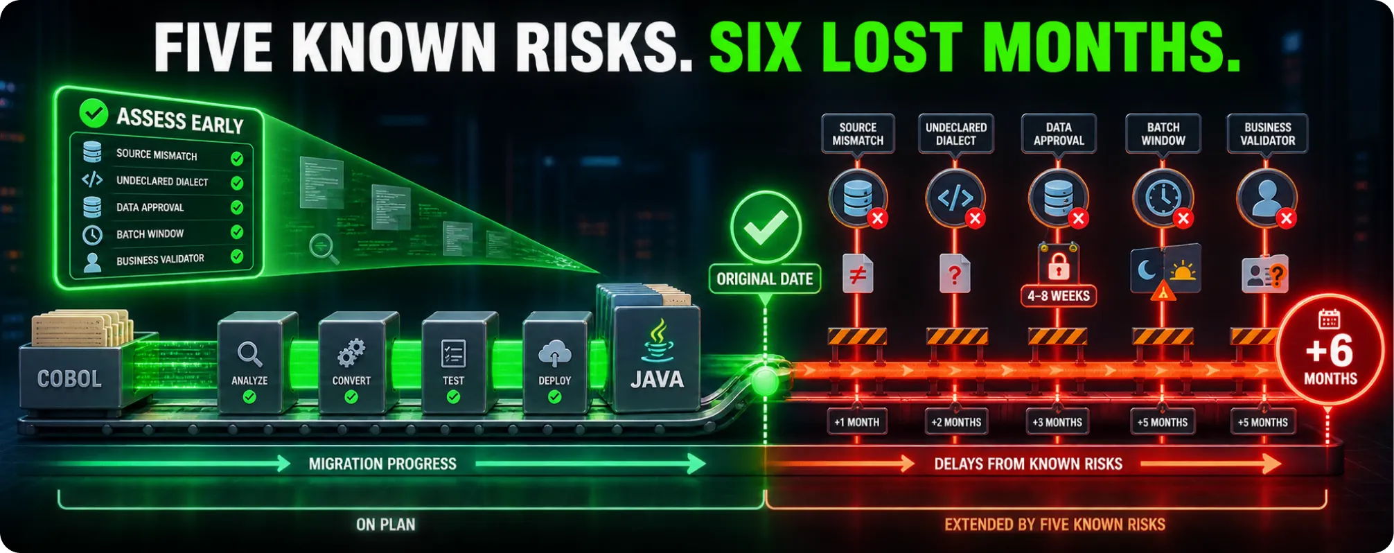
From the pattern across programmes that overrun.
- Source and load module mismatch. Discovered late, this stops everything. The converted system can’t be validated against a source that doesn’t match what’s running. Check this in week 2, not month 14.
- An undeclared dialect. Usually arrives with an acquired system nobody mentioned. Adds front-end work and re-opens the estimate.
- Security review on the production data pathway. Record and replay testing needs production data. In regulated industries that needs approval, and approval takes 4 to 8 weeks that no technical plan includes.
- Batch performance failure at volume. The converted batch runs correctly and misses the window. Found late, this triggers a re-architecture of the batch layer mid-programme.
- Business validator availability. The people who can confirm correct behaviour are the same people running the business. If they aren’t formally allocated with backfill, validation slips every wave.
Every one of these is identifiable during assessment. None of them are technology problems.
What compresses a timeline, and what doesn’t
Compresses:
- Deleting dead code before conversion. If 30% of the estate never executes, converting it is 30% of your conversion and testing budget spent on nothing.
- Fixing the source control situation early. Programmes that discover source and load module mismatches in month 14 lose months.
- Choosing a functional-equivalence target rather than redesigning. You can rearchitect after cutover, on a stable platform, with a test suite that works.
- Deterministic transformation, because rework loops shrink. When the same source produces the same output every time, a rule fix propagates across the whole estate rather than being applied case by case. Semantic Designs’ DMS platform, which fuses symbolic AI with enhanced compiler technology, is built around that property, and the DMS platform page covers the mechanics.
- Gen AI for documentation and test drafting, used as an augmentation layer around the conversion rather than as the conversion itself.
Doesn’t compress, despite the claims:
- Adding conversion capacity. Conversion isn’t the bottleneck, so throwing throughput at it moves work into a testing queue that’s already the constraint.
- Skipping the pilot. Programmes that skip straight to bulk conversion discover their calibration was wrong at scale, and the rework costs more than the pilot would have.
- Generative conversion at scale without a verification plan. Published benchmarks show accuracy falling from above 90% on codebases under 10,000 lines to under 20% above 50,000 lines, and a 2026 study from AWS-affiliated researchers (arXiv:2605.21537) found models detected only 68.3% of their own semantic drift on review. Time saved in generation gets spent, unpredictably, in verification.
What “reliable” looks like on a Gantt chart
One more framing that helps when you’re presenting a timeline to a board.
A modernization schedule has 2 kinds of task: the ones where you can predict the duration, and the ones where you can only predict the duration after you’ve started.
Discovery, conversion and cutover are the first kind. Given a complexity profile, they’re estimable within 20%.
Testing and residual handling are the second kind. Their duration depends on what the conversion produced, and you don’t know that until the pilot.
Presenting a single-line 18-month estimate hides that distinction and sets an expectation you can’t control. Presenting it as a fixed core with 2 calibrated variables sets an expectation you can manage, and it makes the pilot look like what it is: the instrument that removes the uncertainty rather than a delay before the real work.
Boards respond well to this framing. Sponsors who understand which parts of the plan are estimates and which are commitments are considerably less likely to cancel in month 18.
Working out where you sit
A rough self-assessment. Count the yes answers.
- More than 1 COBOL dialect in the estate?
- VSAM or IMS as a primary data store?
- Dynamic CALL used with program names in data fields?
- Embedded assembler anywhere in the execution path?
- No regression test suite that runs unattended?
- Source control uncertainty, or load modules without matching source?
- More than 1 million lines?
- Regulated industry with a formal validation requirement?
0 to 2: you’re likely in the 6 to 12 month band.
3 to 5: 12 to 24 months.
6 or more: plan for 2 years minimum, and structure it in waves with independent business value at each wave boundary.
That last point matters more than the number. A 3-year programme with no deliverable until month 34 will be cancelled in month 18 when the sponsor changes. A 3-year programme that retires a mainframe workload every 6 months keeps funding itself.
We’ve written about that funding dynamic in how to fund modernization when there are no new features at the end.
Does the target language change the timeline?
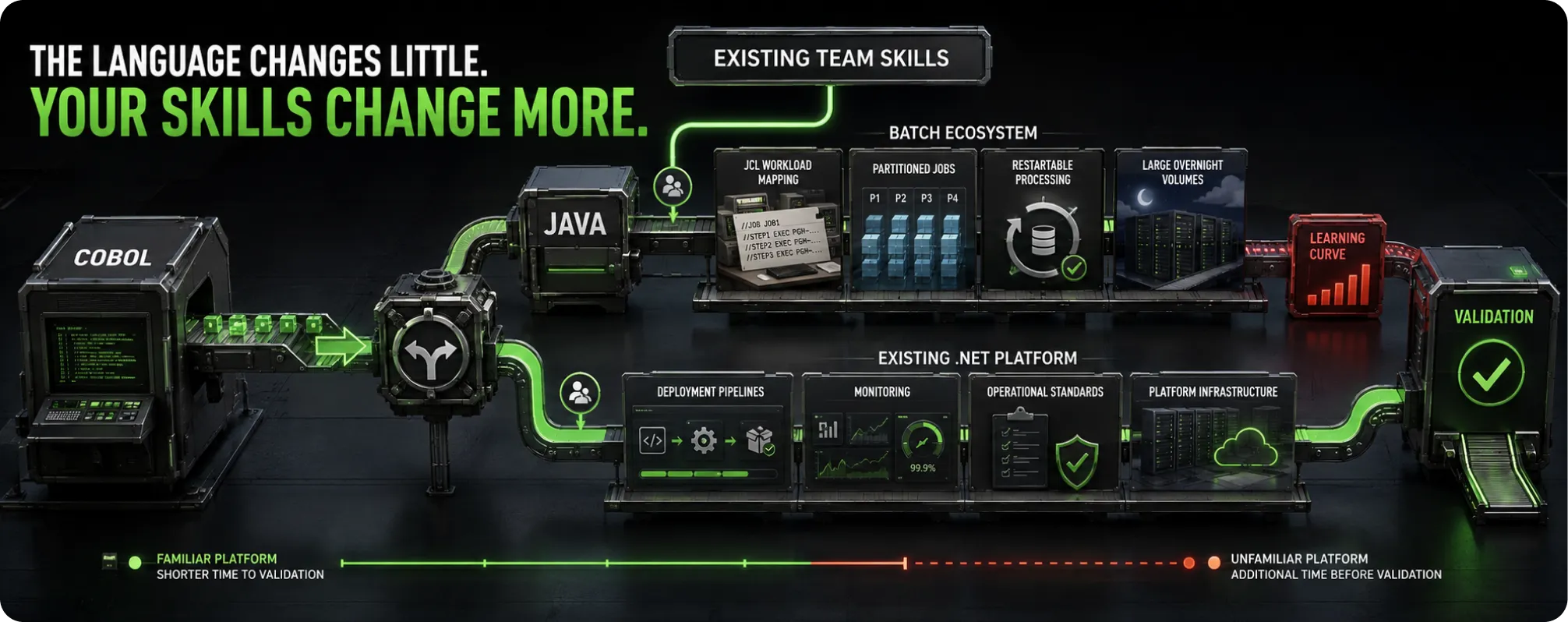
Marginally, and less than people expect.
Java and C# are both mature targets with comparable ecosystems, and the conversion effort is similar. What differs is the surrounding work.
Java has the deeper ecosystem for high-throughput batch processing, which matters on mainframe estates where overnight batch is the dominant workload. Frameworks built for partitioned, restartable batch jobs map reasonably well onto JCL-orchestrated processing.
C# suits organisations already running .NET, because the operational tooling, monitoring and deployment pipelines already exist. That removes weeks of platform setup that a Java target would need from scratch.
The real timeline variable is your existing skills. Converting to a language your team already runs in production removes the platform learning curve from the critical path. Converting to one they don’t adds it to validation, where it costs the most.
Both directions are covered on the COBOL to Java and COBOL to C# pages.
What to fix before you start the clock
Three preparatory items that reliably pay for themselves.
- Reconcile source and load modules. Confirm that what you’re converting is what’s running. Every programme that skips this and finds a mismatch later loses months.
- Eliminate dead code. Analysis identifies what hasn’t executed. Removing 25% of an estate before conversion removes 25% of the conversion, testing and validation effort along with it.
- Allocate business validators formally. Named people, contracted time, backfill arranged. Validation availability is the most common cause of wave slippage and the easiest to solve before the programme starts.
None of these need a vendor. All 3 can be done during procurement, which means they cost you calendar time you were spending anyway.
Frequently asked questions
Can a COBOL to Java migration be done in under 6 months?
Yes, key consideration is afor isolated applications with clean structure and a clear vision for the target architecture, sufficient resources for setting up the target environment and testing , a single dialect and a manageable data layer. Documented examples include 100,000-line conversions completed inside 6 months. Core transaction systems don’t fit this profile.
Does automation cut the timeline in half?
It cuts conversion time dramatically and testing time modestly. Since conversion is 20% to 25% of elapsed time and testing is 25% to 35%, the overall compression is real but smaller than conversion-focused marketing implies.
Why does testing take so long?
Because most legacy estates have no usable regression suite, so the testing phase includes building the oracle you’ll test against. Testhat construction is on the critical path.
Should we convert everything at once?
Almost never above 500,000 lines. Wave-based delivery grouped by subsystem and data dependency lets you validate at a pace the business can absorb and produces value before the programme ends.
What’s the single biggest cause of overrun?
Changes to target architecture and testing. Data migration, followed by discovering complexity that discovery missed. Both are reduced by a properly scoped assessment phase rather than by adding people later.
How long does the assessment itself take?
2 to 8 weeks depending on the complexity of the system and availability of resources to plan the migration and target architecture..architecure.estate condition. It’s a relatively inexpensive investment that can substantially reduce teh project’s risk and accordingly the overall project cost. the cheapest phase and the one that most improves the accuracy of everything after it.
Next step
A timeline you can plan against needs a complexity profile of your actual estate, not a benchmark from someone else’s.
Modernize Software runs a free codebase assessment that produces the inventory, dependency graph and complexity profile a real schedule is built from.
If you’re weighing approaches rather than timelines, four ways to modernize legacy code covers the options, and the COBOL to Java migration page covers how the transformation itself works.
.png)

 info@semanticdesigns.com
